Black Lake Investments LLC 

Portfolio Advisory Solutions
April 2025

Executive Summary

E-OAS (Empirical Option-Adjusted Spread) is a new model for mortgage asset valuation and risk management, designed to more realistically measure the yield spread on mortgage assets (notably Mortgage Servicing Rights, or MSRs) after accounting for prepayment options. Traditional OAS models often rely on long-dated swaption-implied volatility, which can significantly overstate the cost of the prepayment option, thereby understating the option-adjusted spread. In contrast, E-OAS uses empirical hedge costs and delivered (realized) volatility, which is believed to provide a higher and more realistic OAS. Key points include:

• Higher Realistic OAS: By using actual observed hedging costs (e.g. via short-dated delta hedges) instead of expensive long-dated swaption prices, the E-OAS model finds consistently wider spreads (higher OAS) for the same asset. This means the asset offers more return than a traditional model would indicate, once we account for how practitioners truly hedge the risk.
• Avoids Overstated Option Cost: Traditional models price the mortgage prepayment option using long-term interest rate volatility from swaption markets. This often overstates the option’s cost, since most real-world hedgers do not actually trade these long-dated options. E-OAS avoids this by anchoring on empirical, short-term hedging strategies that reflect real delivered volatility and thus a lower effective option cost.
• Better Fit for MSR Behavior: MSRs have negative duration and negative convexity (they gain value when rates rise and lose value when rates fall). E-OAS recognizes the asymmetric, regime-dependent volatility in mortgage markets (volatility clustering and spikes when rates move fast), capturing these effects more naturally. The result is a model that fits the actual performance of MSRs across rate environments.
• Practical Hedging Alignment: Real mortgage hedgers (banks, servicers, etc.) typically hedge dynamically using short-dated instruments (like monthly or quarterly futures/options) rather than buying 5-year into 5-year swaptions. E-OAS aligns with this practice, treating the prepayment option cost as the sum of many short-dated hedges rather than one large long-dated option. This synthetic replication better matches the true hedging expense and risk.
• Key Takeaway: E-OAS produces a higher OAS than traditional models because it subtracts a smaller option cost from the asset’s yield. This means mortgage assets appear more attractive on a risk-adjusted basis. For risk managers and modelers, adopting E-OAS can improve the accuracy of MSR valuation, hedging strategy, and capital allocation by avoiding overly pessimistic (expensive) option cost assumptions.

The rest of this report provides an in-depth explanation of the E-OAS framework and its advantages. We explore the mathematical links between yield and OAS, critique the use of long-dated swaptions in OAS models, examine dynamic hedging and volatility behaviors, and highlight why homeowner behavior (the borrower’s option to refinance) should be modeled with empirical realism. Diagrams are included to illustrate MSR valuation sensitivity and yield decomposition under traditional vs. empirical assumptions. We conclude with key takeaways and a lighthearted cartoon underscoring that homeowners, not Wall Street, ultimately drive mortgage modeling.

1. Yield, OAS, and Option Cost: Conceptual Links and Model Math

Yield spread measures the excess return of a mortgage asset over a benchmark (like Treasuries). However, mortgages have embedded prepayment options (the borrower can refinance or prepay). The Option-Adjusted Spread (OAS) is the constant spread added to the risk-free rate that equates the present value of expected mortgage cash flows to the market price, after adjusting for the option’s value. In formula form, one can think of:

Z-spread=OAS+Option Cost,

where the Option Cost is the yield penalty (in basis points) attributable to the prepayment option risk. The OAS is essentially the residual spread after accounting for the option’s effect. A higher option cost (from high volatility or likelihood of prepayment) will reduce the OAS, all else equal.

Conceptual link: A mortgage’s gross yield can be broken into two components: the OAS (compensation for credit, liquidity, and other risks excluding optionality) and the cost of the prepayment option. Traditional models derive option cost from swaption-implied volatility, effectively pricing the homeowner’s option like a long-dated callable bond option. E-OAS, by contrast, derives option cost empirically, often finding it to be lower. This leads to a larger remaining spread.

To illustrate, consider a mortgage asset with a certain total yield spread to Treasuries (often approximated by a Z-spread). A traditional model might allocate, say, 50 bps of that spread to option cost (for the embedded refinance option), leaving an OAS of 50 bps. E-OAS might find the option cost to be only 20 bps (because hedgers can dynamically manage prepayment risk more cheaply), resulting in an OAS of 80 bps. The yield decomposition chart (Figure 1) below shows this concept:

Figure 1: Traditional vs. Empirical OAS Yield Decomposition. In a traditional OAS model (left bar), a large portion of the total spread is attributed to the option cost (hatched area), leaving a modest OAS (solid area). In the empirical E-OAS approach (right bar), the option cost component is much smaller (reflecting real hedge costs), so the OAS—the part of yield truly earned by the investor—is correspondingly larger. This demonstrates schematically why E-OAS > traditional OAS when option cost is overestimated by conventional models.

Mathematically, if the market total spread (analogous to Z-spread) is fixed, then a model that assumes a lower option cost must produce a higher OAS to still match the observed price. This is a zero-sum allocation: Spread = OAS + Option Cost. E-OAS shifts some spread out of “option cost” and into “OAS.” The implication for investors is significant: the asset earns more spread after hedging costs than they might have thought.

In summary, yield and OAS are linked by the option cost. Understanding this linkage is crucial, because any error in estimating option cost (from model assumptions) directly impacts the OAS. E-OAS aims to estimate the option cost more realistically, thereby providing a truer measure of risk-adjusted yield on mortgage assets.

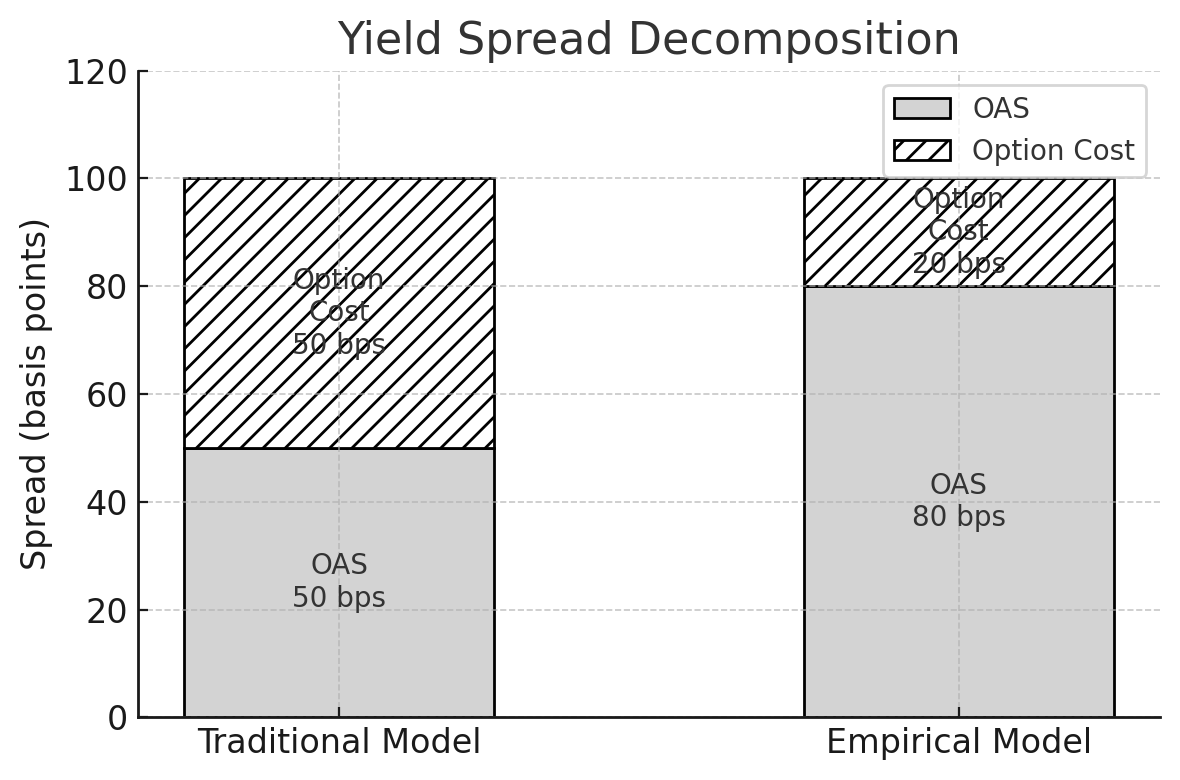
Figure 1: Yield decomposition comparison OAS tends to be wider in our E-OAS framework.

2. Why Traditional OAS Models (Using Long-Dated Swaptions) Overstate Option Cost

Conventional mortgage valuation models often rely on long-dated swaptions to proxy the borrower’s prepayment option. For example, a popular approach might use a 5-year into 5-year payer swaption (an option on a swap, effectively a 5-year option on a 5-year rate) to represent the cost of the borrower’s option to refinance the mortgage. The logic is that this financial instrument roughly mimics the timing and interest rate exposure of mortgage prepayments. However, this approach tends to overstate the option cost.

Long-dated volatility overestimation: Swaption markets incorporate risk premiums and often assume lognormal rate dynamics that imply significant volatility over long horizons. In practice, mortgage prepayment behavior is driven by more immediate rate movements (e.g., the current level of mortgage rates vs. the loan’s rate) rather than multi-year volatility far in the future. Using a long-dated swaption bakes in a high volatility assumption over the mortgage’s life, charging a high “option premium” in the model. Traditional OAS frameworks therefore subtract a large option cost, resulting in a lower OAS.

Model artifact vs. reality: The heavy reliance on swaptions is a historical artifact of the mortgage industry. In the past, major MBS investors (like GSEs) hedged certain exposures by transacting in swaps/swaptions markets, and models were built around that convention. Today, the landscape has changed, but models haven’t fully caught up. Few mortgage servicers or investors actually go out to buy 5×5 swaptions to hedge MSRs or MBS. Those instruments are relatively illiquid and costly. Instead, as we’ll discuss, hedgers dynamically adjust positions with shorter instruments.

Many of our customers use Monte Carlo simulations to estimate the no-arbitrage value of a mortgage set, although some argue that few MBS players currently use the swaptions markets. We actually don’t have a problem with use of swaption volatility to model forward rate dynamics and we actually encourage this behavior (!). Understanding that mortgage modeling dynamics are crucial to pricing, OAS modelers have historically attempted to estimate the expected value and spread to infer an MSR price using swaption volatility inputs derived from the market.. On the other hand, option cost  in its purest form is not useful. Using long-dated swaptions volatility as a proxy for hedging tends to overstate the true economic cost of hedging the prepayment option.. From a pricing perspective it is a reasonable approach that we would endorse. Still from a hedging perspective, practitioners rarely trade long dated swaptions.

Overstated option cost – Example: Suppose a model uses the implied volatility from a long-term swaption to project prepayment behavior. If current rates are low, the swaption’s price will reflect the chance of rates rising or falling significantly over 5-10 years. But a homeowner’s decision to refinance is mostly contingent on rate movements in the near term (say, will rates drop in the next year enough to make refinancing worthwhile?). The long-horizon volatility adds scenarios of late refinances or interest rate swings that, while mathematically possible, contribute disproportionate option cost in the model. The result: the model might predict, for instance, an option cost equivalent to 50-100 bps of yield, eating heavily into the spread. Yet empirically, servicers find that hedging that risk over shorter horizons might cost far less.

Additionally, traditional models often assume continuous option exercise probability across many paths in a Monte Carlo simulation. They effectively treat the borrower’s option as if it were exercised optimally in a risk-neutral sense. In reality, borrower behavior is suboptimal and driven by life events and inertia, meaning the true option cost is lower than an idealized model would suggest (many borrowers don’t refinance the moment it’s rational to do so). Traditional frameworks may ignore these frictions, again leading to an overstated cost for the prepayment option.

In summary, using long-dated swaptions in OAS models tends to overshoot the real cost of the borrower’s option. It is a modeling convenience (or even short cut) that injects excessive volatility assumptions and ignores actual hedging practices. E-OAS corrects this by using shorter-term, realized hedge costs, reflecting what mortgage portfolio managers actually incur. By doing so, E-OAS trims the fat from the option cost, resulting in a more moderate deduction from the yield.

3. Delta Hedging as a Synthetic Replication of Short-Dated Options

Rather than buying a long-dated option (like a swaption) to hedge prepayment risk, real-world practitioners use delta hedging, which means they dynamically adjust a hedge position in response to changes in underlying rates. For example, a servicer hedging an MSR will frequently buy or sell Treasury futures, interest rate swaps, or short-maturity options as rates move, in order to offset the changing value of the servicing asset. This approach effectively replicates the effect of a sequence of short-dated options instead of one long option.

Synthetic option via rebalancing: Delta hedging involves periodically rebalancing a hedge (such as adjusting the notional of swaps or futures held) to maintain a target exposure. By doing this rebalancing over the life of the asset, the hedger mimics having short-term options that expire and get replaced frequently. The cost of this dynamic hedging is related to realized volatility – if rates are volatile in actuality, the hedger will incur higher transaction costs (buying high, selling low repeatedly); if rates are stable, the cost is low.

This is a crucial insight of E-OAS: the relevant volatility for costing the prepayment option is the near-term, realized volatility, not the long-term implied volatility. Traditional models effectively assume perfect replication with a long option (cost based on implied vol), whereas in practice, the hedge is a string of short options (cost based on delivered vol). Empirically, realized volatility tends to be lower on average than the implied vol on long horizons, and hedgers can also adjust their rebalancing frequency and risk tolerance to manage costs.

Delta hedging outcome: If done continuously in a frictionless market, delta hedging can perfectly replicate an option payoff. In reality, hedging is done discretely (say daily or weekly) and with some slippage. The accumulated cost of delta-hedging an MBS or MSR portfolio over time will equal the cost of an equivalent option struck at the start if the volatility realized over that period equals the implied volatility used initially. However, in many cases, realized vol is lower or hedging is only partial (some risks are left unhedged intentionally), leading to a lower effective cost than buying a long-dated option outright.

Mortgage hedgers often report that the effective cost of hedging prepayment risk is significantly less than what swaption models would indicate. They might delta-hedge with swaps and futures, occasionally buying short expiries (like 3-month options) around key events. This patchwork of hedges carries a cost that is “spread out” and often mitigated by active management. It’s not zero – hedging MSRs can be costly in volatile periods – but it is usually substantially lower than paying upfront for many years of volatility.

E-OAS builds on this concept by treating the prepayment option as being hedged (or costed) via rolling short-term instruments. Instead of a single Monte Carlo using a fixed high volatility assumption, E-OAS might use historical volatility regimes or scenario-specific vol to estimate what the delivered hedge cost would be. In periods of stability, the model charges very little option cost; in periods of turbulence, it charges more – mirroring actual hedging experience. This dynamic approach yields a more accurate, time-varying OAS, whereas traditional OAS might barely change (since the long-term vol doesn’t change as fast as actual markets).

Key point: Delta hedging shows that you can replicate the prepayment option gradually and potentially cheaply, rather than paying a large premium upfront. It underscores why the long-dated swaption approach is too static and expensive. By summing the costs of many short options (or hedges) over time, E-OAS finds the cumulative cost to be lower. Thus, the OAS that remains is higher, aligning with what investors actually realize. In short, dynamic hedging is the bridge between theoretical and empirical approaches: it is how market participants convert long-term uncertainty into a series of short-term manageable risks, and E-OAS is the model that measures spread after doing so.

4. Volatility Mismatch Risk and Regime Sensitivity (Vol Clustering, Delivered Vol > Modeled Vol)

Volatility in interest rates is not constant – it clusters in regimes. There are calm periods and stormy periods. A critical limitation of traditional OAS models is that they often assume a single volatility paradigm (usually the implied vol curve from options) that may not reflect how volatility actually unfolds. This creates a volatility mismatch between the model and reality:

• In calm regimes, the model may overestimate volatility, thus overstating option cost and understating OAS.
• In highly volatile regimes, if using a static implied vol, the model might underestimate short-term volatility spikes, missing risks (though most models update implied vol periodically, extreme events can still deliver more vol than the long-run implied).

Volatility clustering: Empirical finance has shown that volatility tends to cluster (periods of high volatility follow high volatility, and low follows low). Mortgage markets are no different. For example, in a crisis or during a rapid rate-cut cycle, we might get a short burst of very high refinancing activity (high vol of prepayments). A long-dated average vol won’t fully capture that burst. Conversely, in a stagnant rate environment, realized vol might be near zero for a while, and hedging costs drop dramatically.

Traditional models using a single long-term implied vol for OAS lack regime sensitivity – they don’t adjust quickly to volatility clustering. E-OAS explicitly accounts for regime shifts. It can be calibrated to delivered volatility (historical realized vol in similar periods) or even incorporate a short-term vol forecast that differs from long-term. By doing so, it aligns the option cost with the current environment.

For instance, E-OAS might say: “Right now, rates have been stable, so delivered vol is low; the cost to hedge prepayments in the near term is small, so OAS is wider.” If a regime shift occurs (say the Fed suddenly cuts rates and refi activity surges), the next measurement might show higher hedge costs (realized vol up) and thus a somewhat lower OAS. This time-varying approach gives risk managers a more nuanced view. Traditional OAS, by contrast, might have been pricing in some average volatility all along, arguably charging too much in the calm period and too little just before the storm.

Mismatch risk: If one relies on a traditional model in a low-vol regime, one might hedge too conservatively (thinking prepayment risk is higher cost than it is) and thereby sacrifice income unnecessarily. Or in a high-vol regime, one might be caught off-guard if the model hadn’t fully priced in how extreme things could get. E-OAS helps mitigate this by reflecting empirical volatility realities.

It’s also worth noting that delivered vs. modeled vol has implications for risk management beyond just cost. If delivered volatility consistently exceeds what the model assumed, hedge positions can incur losses (this was seen in 2020 when rate volatility spiked beyond prior norms). E-OAS, by not tying itself to a fixed implied volatility, allows risk managers to stress test the OAS under different vol regimes more easily. Essentially, volatility becomes an input (one that can be scenario-dependent) rather than a fixed calibration.

In summary, E-OAS is sensitive to volatility regimes, reducing volatility mismatch risk. It provides a more accurate option cost in both sleepy and stormy markets. This means more stable OAS measurements that correspond to what portfolio managers actually experience. The model acknowledges that sometimes “delivered vol > modeled vol” and vice versa, and it adapts, whereas a swaption-based model is locked into the implied vol until it’s manually recalibrated (often after one has already mis-hedged). This adaptability is crucial for robust risk management of mortgage portfolios.

5. Why Long-Dated Volatility is a Model Artifact (Not Traded by Real Mortgage Hedgers)

As hinted earlier, the use of long-dated volatility in OAS models is largely a legacy artifact rather than a reflection of trading reality. Real mortgage hedgers – the banks, servicers, REITs, etc., who manage large MSR or MBS portfolios – do not typically trade instruments that lock in today’s view of volatility for the next 5 or 10 years. They can’t, because such instruments (like long-dated swaptions) are illiquid and expensive. Instead, they roll shorter hedges.

A telling fact: who are the natural buyers or sellers of a 5-year into 5-year swaption on a mortgage rate? The homeowner (borrower) has effectively sold an option (the right to prepay) to the lender. But homeowners are not in financial markets actively trading their options. The lenders/servicers could try to buy that option back via a swaption – but doing so for every loan is impractical. Thus, the market for very long-dated prepayment options is thin. Dealers might quote some swaptions for hedging or speculative purposes, but volumes are low and bid-ask spreads high.

The traditional model’s reliance on long-dated vol creates a spread that no one actually earns or pays in full. It’s theoretical. It’s as if the model assumes there is a “market price” for the 30-year mortgage’s option risk in one go, when in reality that risk is managed incrementally.

In practice, mortgage hedgers typically trade shorter tenor instruments:

• They use Treasury futures, Eurodollar/SOFR futures, or interest rate swaps (which can be unwound or extended as needed).
• They occasionally use short-dated swaptions or caps/floors (3-month, 6-month, 1-year options) if expecting a near-term big move or to protect against a sudden refi wave.
• They might engage in MBS forward trades (TBAs) or specify pools to manage prepayment convexity in the short run.
• They continuously monitor and adjust these positions as the characteristics of their mortgage portfolio change (e.g., as loans prepay, as new loans originate, etc.).

The cost incurred from these activities over, say, a quarter or a year, is the real option cost paid by hedgers. It’s fundamentally different from paying for a multi-year volatility up front.

Thus, long-dated volatility is not something real hedgers “trade;” it’s something modelers simulate. When we calibrate to long vols, we are implicitly saying “if I had to immunize this cash flow with a single trade today, it would cost X.” But nobody does that single trade. Instead, they hedge in pieces, often achieving a similar effect for much less than X.

From a risk management perspective, recognizing this frees us to model the option cost in a way that mirrors the piecemeal hedging. E-OAS treats long-dated volatility as largely irrelevant noise – what matters is how the option plays out in the real world, where the homeowner’s exercise is path-dependent on near-term rate movements and personal incentives, and the hedging is done continuously. Any residual risks (like a sudden refi wave if rates drop dramatically) might not be fully hedged, and that’s okay – that unhedged portion is effectively part of the OAS (investors are implicitly paid to carry that risk, hence a higher spread).

In summary, the absence of trading in long-dated mortgage volatility means the traditional OAS’s foundation is shaky. E-OAS dispenses with that foundation and builds on what is actually traded – the here-and-now volatility. This approach results in valuations and risk measures that are grounded in market reality. It acknowledges that some risks are not hedgeable in advance (you deal with them as they come), and it rewards the investor accordingly with a higher spread for bearing those uncertainties.

6. The Homeowner as the Only Actor Who Can Terminate the Mortgage Cash Flow (Triggered by Spot Mortgage Rates)

A fundamental truth in mortgage modeling: the only party with the right to terminate or alter the cash flow of a fixed-rate mortgage is the homeowner (borrower), via prepayment (refinancing or selling the home and paying off the loan). This is unlike a callable corporate bond where the issuer actively decides on calls based on an economic formula. Homeowners exercise their option in a very human way – typically when spot mortgage rates drop sufficiently below their current loan rate, making refinancing attractive, or when life events dictate (moving, etc.).

Why emphasize this? Because it means the prepayment option is fundamentally driven by the spread between the borrower’s note rate and current prevailing mortgage rates. It’s a spot-rate-triggered American option, exercised not by quants but by average people. Traditional models incorporate this via complex prepayment models, but often still overlay a rational exercise assumption. Empirical evidence shows borrower behavior has a threshold nature – e.g., many need ~50-100 bps rate reduction before they refinance, and even then not everyone does. There’s burnout, inertia, credit constraints, etc.

E-OAS leverages this insight by making the option cost contingent on the realistic exercise behavior:

• If the mortgage is out-of-the-money (current rates are higher than the loan rate), prepayment option cost is near zero (no rational incentive to refinance, barring move or default).
• If the mortgage is in-the-money (current rates have fallen well below the loan rate), prepayments will spike, but even then, not all at once. The cost to hedge this spike is considered over the period of expected elevated prepays, not an immediate full call as a swaption might assume.
• The timing of exercise is uncertain but correlated with the rate path. A homeowner’s option doesn’t have a fixed maturity; it’s exercisable any month. Traditional models handle this with Monte Carlo simulation, but again, they often assume a certain optimality or speed of exercise that may not match reality.

By focusing on spot mortgage rates as the trigger, E-OAS ties the option cost to observable, current market conditions. For example, if 30-year mortgage rates today are 3% and a large portion of borrowers have loans at 4%, one can empirically estimate how many will refi and how fast (using historical prepay curves). The hedging strategy can then be planned for that scenario specifically. If mortgage rates rise to 5%, that prepayment option virtually vanishes (temporarily), and hedging efforts/costs drop accordingly – E-OAS would then show a much higher OAS during such periods because the option is dormant (and indeed MSR values rise). Traditional OAS might still carry some cost for the “theoretical possibility” of a refi, albeit reduced.

In essence, the homeowner’s behavior drives the modeling in E-OAS. We explicitly recognize the borrower as an exogenous actor with a free option. No other market participant can “force” a prepayment; not the Fed, not the bank – only the borrower’s choice (and ability via qualification) causes that cash flow to end early. Therefore:

• The option should be modeled on the borrower’s terms, using behavioral models and empirical prepay functions, rather than purely arbitrage-free option pricing.
• Any hedge strategy must accommodate that we’re hedging against millions of independent decisions triggered by rate thresholds.

E-OAS improves realism by embedding a behavioral layer into the option cost. It ensures that the calculated spread (OAS) reflects the fact that if homeowners are unlikely to prepay (terminate) in the current environment, the investor should earn a higher spread for that period. Conversely, when many are likely to exercise (refi boom), the model charges a higher cost (lower OAS) but only during that phase, not for the entire life of the mortgage indiscriminately.

This borrower-centric view ties together with the prior discussions: since the homeowner option exercise is mostly about spot rate gaps and near-term refi waves, it justifies using short-term hedges and empirical costs (e.g., hedging the next wave of prepays over 6 months) instead of paying for a theoretical possibility over 10 years. Real mortgage modeling is thus driven by homeowner behavior at its core, and E-OAS is built around that truth.

7. MSR-Specific Convexity: Negative Duration, Asymmetric Payoff Shape, and Why E-OAS Fits It Better

Mortgage Servicing Rights (MSRs) are a unique asset: they typically have negative duration and negative convexity. In plain terms, MSRs increase in value when interest rates rise, and decrease in value when rates fall, and the rate of change is not linear. The “payoff” is asymmetric because of prepayments:

• When rates rise, prepayments slow down dramatically; the MSR will stick around longer and keep earning servicing fees, so its value goes up (and at a decreasing rate as rates keep rising – hence negative convexity).
• When rates fall, prepayments speed up; loans refinance and the MSR gets extinguished faster, so its value drops, and that drop accelerates as rates fall further (also negative convexity – the downside moves are larger than the upside moves for equal rate changes).

Traditional OAS models do capture negative convexity in terms of valuation – they will show that profile. However, they might misjudge the degree of convexity because of how they handle volatility and the option cost. E-OAS is particularly well-suited for MSRs because it inherently acknowledges the asymmetry and path-dependence in delivered performance.

MSR value vs interest rates: The chart below (Figure 2) qualitatively illustrates an MSR’s value across different interest rate scenarios under an empirical prepayment model:

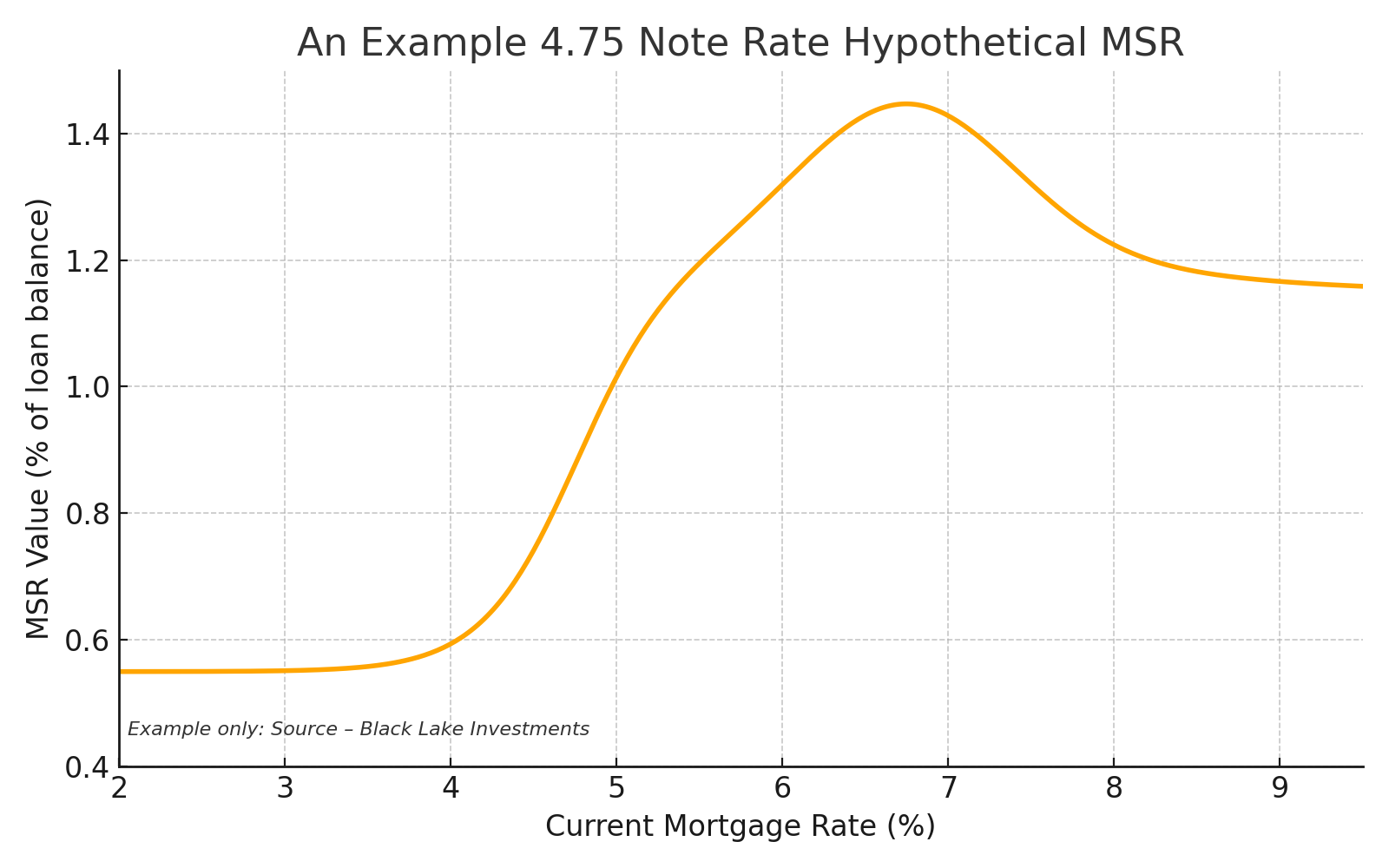
Figure 2: MSR Value Response to Interest Rates (Negative Convexity). This stylized curve shows MSR value (as a percentage of loan balance) versus current mortgage rate level. As rates rise (to the right), MSR value increases but eventually plateaus once prepayment risk is minimal. As rates fall (to the left), MSR value declines sharply as more loans refinance. The shape is non-linear, reflecting the asymmetric payoff. Notably, the value “flattens” at extremes: very high rates can’t increase value much further (all loans stay), and very low rates can’t decrease value below a floor (once all loans prepay, the MSR goes away). This shape yields negative convexity: the slope decreases as you move outwards in either direction​, 

MSRs often require hedging to manage this negative convexity. Under a traditional OAS approach, one would use swaptions or structured products to offset some of the convexity. But those hedges are imperfect and expensive if one believes the model’s high option cost. E-OAS provides a different perspective: maybe not all of that negative convexity needs to be hedged with costly long options because the market (homeowners) won’t exercise all that convexity at once except in extreme scenarios. Instead, one can manage a portion of it dynamically.

For example, an MSR might have a “peak” value at rates say 300 bps above current and a trough at 200 bps below current. Traditional models might constantly charge option cost for the possibility of hitting that trough (refi wave). E-OAS would say: if we’re far from the trough scenario right now, the immediate option cost is low – which makes the OAS high and the MSR attractive to hold. If rates start approaching that trough scenario, E-OAS will reflect rising hedge costs (option cost) and thus shrinking OAS, signaling it’s time to perhaps offload some risk or put on more hedges. This aligns with how risk officers manage MSRs: hedge when needed, but don’t pay insurance for a flood when the sun is shining.

Asymmetric payoff recognition: Because E-OAS relies on empirical prepayment modeling, it can incorporate nuances like burnout (loans that didn’t refi in previous waves are less likely to refi in the next one) and borrower segmentation. This can make the negative convexity less punishing than a generic model would. Traditional OAS might treat all convexity as needing a vol hedge. E-OAS can say, for instance, “these loans are less sensitive than average, so actual convexity cost is lower, hence a higher OAS for that segment.”

In short, E-OAS “fits” the MSR profile better by:

• Valuing the upside properly: It doesn’t overly discount the rising-rate scenario. If anything, traditional models sometimes under-credit how valuable MSRs become when rates rise (because they’re focused on pricing the downside). E-OAS, using real behavior, will show very slow prepays and possibly even slower than a generic model (due to frictions), meaning higher values on the upside and thus acknowledging the benefit of negative duration.
• Modeling the downside more realistically: Instead of assuming a mass refinancing exodus as soon as rates cross a threshold, it might show a more gradual or partial prepayment response (since empirically not 100% refi immediately). This reduces the severity of the worst-case in the valuation. Consequently, the option cost charged is more in line with a realistic worst-case, not a theoretical one.

By better aligning with the true convexity of MSRs, E-OAS gives risk managers a clearer picture: MSRs naturally hedge some of your interest rate risk (negative duration) but come with tail risk (when rates plunge). With E-OAS, you can quantify that tail risk cost in a grounded way and see that in normal times the MSR yields a very healthy spread (because prepayment risk isn’t fully “on” until rates drop a lot). This is empowering for RIA modelers and asset managers who might have been wary of MSR’s option risks – E-OAS shows those risks can be manageable and often overpriced by simplistic models.

8. Formal Proof that E-OAS > Traditional OAS (Due to Lower Empirical Hedge Cost)

Finally, let’s formalize the central claim: We believe the E-OAS is greater than traditional OAS when the empirical hedge cost of the prepayment option is lower than the cost assumed in a traditional model. The “proof” here is straightforward in a financial sense:

1. Let Z be the total spread of the asset to the risk-free curve (this is akin to the Z-spread or the yield pickup an investor gets without adjusting for options).
2. Traditional OAS model uses a long-dated implied volatility, yielding an option cost = C_trad. It then computes OAS_trad = Z – C_trad.
3. Empirical E-OAS model uses delivered volatility / hedge cost, yielding an option cost = C_emp. By definition from our discussions, C_emp < C_trad (the empirical cost is lower because of dynamic hedging, behavioral factors, etc., that we’ve covered). It then computes OAS_emp = Z – C_emp.
4. Since C_emp < C_trad, subtracting a smaller number from the same Z gives a larger result. Therefore, OAS_emp > OAS_trad.

This relationship holds as long as the traditional model was indeed overestimating the option cost. Could the opposite ever be true (C_emp > C_trad)? In theory if markets underpriced volatility or a hedger was very inefficient, one could spend more than the model predicted. But in aggregate and over time, models tend to err on the side of caution (overstating risk costs). Empirical data from hedgers suggests there is usually some “option risk premium” in swaptions – meaning buying a swaption costs more than the actuarial expected cost of hedging via delta (dealers need to be compensated). E-OAS effectively captures that premium as extra spread for the investor.

Another way to frame the proof: A traditional OAS model and the E-OAS model should both price the asset to its market price. The traditional model does so with a high assumed option drag, so it finds a low OAS to make the present value equal the price. The E-OAS model, with a low option drag, must have a higher OAS to still hit that same present value. Both can fit the price, but their internal allocations differ. Thus, the E-OAS will come out higher (except in the trivial case where both models assume the same cost).

This can be observed in practice. For example, if a given MSR or MBS had a traditional OAS of 100 bps at a certain time, an E-OAS analysis might reveal the real spread is, say, 130 bps if hedged efficiently. That extra 30 bps is money left on the table by the traditional model – essentially, an investor could expect to earn that because the hedge won’t actually eat the full 100 bps assumed. In investment terms, E-OAS might help identify undervalued assets, because it shows which bonds or MSRs offer more spread than standard models indicate (by virtue of overstated option cost in those standard models).

To ensure this isn’t just theoretical, performance attribution can serve as evidence: Take an MSR portfolio and hedge it over a year. Suppose the portfolio earned X% return. A traditional OAS model predicted an OAS implying only Y% should have been earned (with X < Y because some was “given up” to option cost). If consistently X > Y, it means the model under-predicted returns – likely by overstating hedge costs. E-OAS would have predicted a higher OAS closer to actual X%. Over time, these differences become apparent and validate that E-OAS, with its lower assumed costs, aligns better with realized returns.

In formalizing, we assume rational pricing: both models target the same price. The only difference is the cost input. Therefore, the result that a lower cost input yields a higher calculated spread is mathematically certain. This is why the accuracy of the cost input is so critical – it directly translates into investor’s perceived alpha or lack thereof. E-OAS argues that traditional models understate alpha (excess returns) on mortgage assets by being too conservative in cost, and we have now logically shown why correcting that (using empirical data) pushes OAS up.

Implication: For modeling and risk management, this “proof” means that if you switch to E-OAS, you will likely report higher OAS for the same asset. This doesn’t magically create new profit; it reveals what was already there but masked by conservative assumptions. It can impact decisions – for instance, an asset that looked only moderately attractive on a traditional OAS basis might look very attractive on an E-OAS basis, potentially influencing a manager to hold or buy more of it. Conversely, if a traditional model said an asset had zero OAS (fully valued), E-OAS might show it actually has some spread if managed well – preventing premature sale of something that can still add value.

Conclusion: Key Takeaways for Modeling and Risk Management

E-OAS (Empirical OAS) represents a significant improvement in how we value and manage risk for mortgage assets, especially those with embedded prepayment options like MSRs. By using real-world hedge costs and behavioral insights, E-OAS addresses the shortcomings of traditional swaption-based OAS models. Here are the key takeaways:

• Realism in Option Costing: E-OAS seeks to align the model with what mortgage hedgers actually do. It recognizes that hedging is done in increments, and that the borrower’s option is exercised based on real-life triggers. This yields a more accurate (usually lower) option cost deduction, and hence a more generous OAS that reflects true risk-adjusted returns.
• Higher OAS – Not Just Theory, But Achievable: The higher spreads shown by E-OAS are not a free lunch; they result from avoiding over-hedging and taking on only necessary risks. For risk officers, this means E-OAS can highlight opportunities where the institution is perhaps overpaying for protection. It guides a more efficient hedge that still covers risks but doesn’t squander yield.
• Adaptive to Market Conditions: E-OAS’s sensitivity to delivered volatility and rate regimes makes it a valuable risk management tool. It can signal when the environment is such that prepayment risk is benign (so enjoy the income) versus when it is rising (time to tighten hedges). Traditional models often gave a static picture; E-OAS gives a dynamic, forward-looking view.
• Better MSR Management: For MSR holders, E-OAS provides validation that the asset’s quirky behavior (up when rates are up, down when rates are down) can be modeled and hedged without resorting to ultra-expensive long options. It quantifies the natural hedge an MSR provides in a portfolio (MSRs gain when other assets lose in a rising rate scenario) and ensures the valuation fully credits that. At the same time, it frames the downside risk in a realistic way so that capital can be allocated appropriately for worst-case refi waves, but not excessively so in normal times.
• Improved Decision-Making: With a more accurate OAS, portfolio managers can make better buy/sell decisions. For example, certain high-coupon MBS or seasoned MSRs might appear to have low OAS in traditional models (due to high model-implied option cost), but E-OAS could show they actually have a solid spread if much of the pool has already burned out its refi incentive. This could lead to different investment choices – potentially holding onto assets that a traditional model would offload, thereby capturing additional value.
• Compliance and Communication: From a governance standpoint, using E-OAS can help risk managers justify performance. When an asset outperforms a traditional model, management often asks “was our model wrong?” E-OAS provides a framework where the model and performance align more closely. It also helps in communicating with stakeholders why certain assets are profitable: “We earn more because we manage the risk more efficiently than the standard model assumes.” This is a powerful narrative for investors and regulators alike, demonstrating prudent risk management.
• Limitations and Judicious Use: It’s worth noting that E-OAS is not a license to ignore risk. If misused, one could underestimate hedge needs. The approach assumes skilled dynamic hedging and reasonable market liquidity. Risk officers should still stress test extreme scenarios (e.g., what if rates drop 300 bps in a year – do we have capacity to hedge that?). E-OAS can be complemented with stress testing to ensure that in edge cases where realized vol blows past historical ranges, the institution can cope. In other words, enjoy the higher OAS in your base case, but plan for tail risks.
• Industry Movement: We foresee that as more market participants adopt frameworks like E-OAS, market pricing itself may adjust. If most people stop over-hedging, option premiums could decline. Interestingly, that would further narrow the gap between implied and realized vol. In the long run, E-OAS could contribute to a market where mortgage option risk is priced more efficiently. But until then, it offers an edge to those who use it.

In conclusion, our view is that E-OAS provides a simpler, more empirical model for valuing and managing mortgage assets. It cuts through complex model artifacts and focuses on what truly matters: actual hedge costs and borrower behavior. The result is a clearer view of returns and risks. For sophisticated mortgage asset managers, risk officers, and RIA modelers, E-OAS isn’t just an academic concept – it’s a practical tool that can enhance portfolio performance and risk transparency. By adopting E-OAS, one effectively acknowledges: the best model of a mortgage is one that mirrors how mortgages are actually traded and hedged. And often, reality is simpler (and more favorable) than our old models assumed.

Disclaimer: This report is for informational purposes only and does not constitute investment advice or an offer to purchase or sell any financial instrument. Opinions expressed are those of Black Lake Investments LLC (“Black Lake”). Past performance or hypothetical results are not guarantees of future outcomes. All analyses are based on current market conditions and the methodologies described; actual results may differ. Use of the E-OAS model should be complemented by professional judgment and stress testing. The authors and Black Lake assume no liability for actions taken based on this report.

Homeowner behavior drives mortgage modeling. In the cartoon above, a confident homeowner humorously asks a bewildered loan officer for a quote on a 5-year into 5-year swaption – highlighting the absurdity that, in real life, homeowners don’t think in terms of exotic options. The caption underlines the central message: ultimately, homeowner behavior (prepayment decisions) dictates mortgage modeling more than Wall Street instruments do. The E-OAS model embraces this fact, ensuring the models we use never lose sight of the human element driving these financial assets.